
A Practical Test of the Low-Volatility Anomaly in U.S. Equities (2020–2025)
Challenging the risk-return paradigm
In this article, I examine whether low-volatility stocks can deliver returns comparable to — or even exceeding — those of the benchmark, but with significantly less risk. Using QuantConnect, I implement a systematic, monthly rebalanced strategy that selects the 30 least volatile equities from the 500 most liquid U.S. stocks. I use SPY as the benchmark for comparison.
The result?
Improved Sharpe ratio compared to SPY
Reduced drawdowns and a smoother equity curve
Market-like returns with lower volatility
This outcome challenges the traditional financial paradigm that higher returns require higher risk, and supports the anomaly first documented by Ang et al. (2006).
1. Low Risk, Still Rewarded
Classical financial theory posits that investors must accept higher risk to earn higher returns. However, empirical studies suggest the opposite: stocks with lower historical volatility tend to outperform on a risk-adjusted basis — and sometimes even in absolute terms.
“Low volatility doesn’t mean low return — it means lower regret.”
— Pim Van Vliet, PhD, portfolio manager
This strategy investigates whether that effect holds in U.S. equities from 2020 to 2025, using a universe that mirrors the benchmark.
2. Strategy Implementation: Systematic Volatility Selection
Universe: Top 500 U.S. stocks by average daily dollar volume, filtered for price > $5
Signal: Annualized volatility computed from the trailing 3 months (60 trading days)
Selection: Each month, select the 30 stocks with the lowest volatility
Rebalancing: Monthly — executed on the first Monday at 10:00 AM
Portfolio Construction: Equal-weighted allocation
Risk Management: 5% trailing stop-loss per security and 10% drawdown cap at the portfolio level
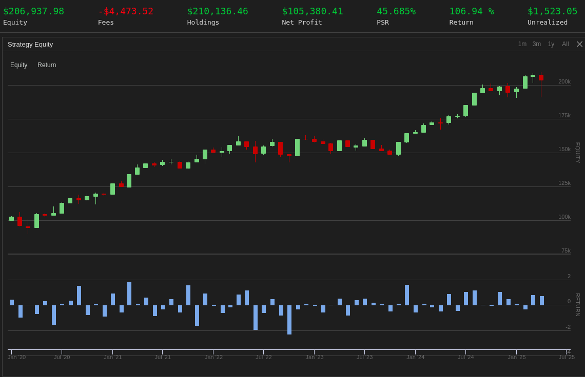
3. Results (Backtest: 2020–2025)
SPY serves as the benchmark, delivering an 88% return over the period, with a Sharpe ratio of 0.42 and a CAGR of 12.6%. Its maximum drawdown — during the COVID-19 crash — reached 33%.
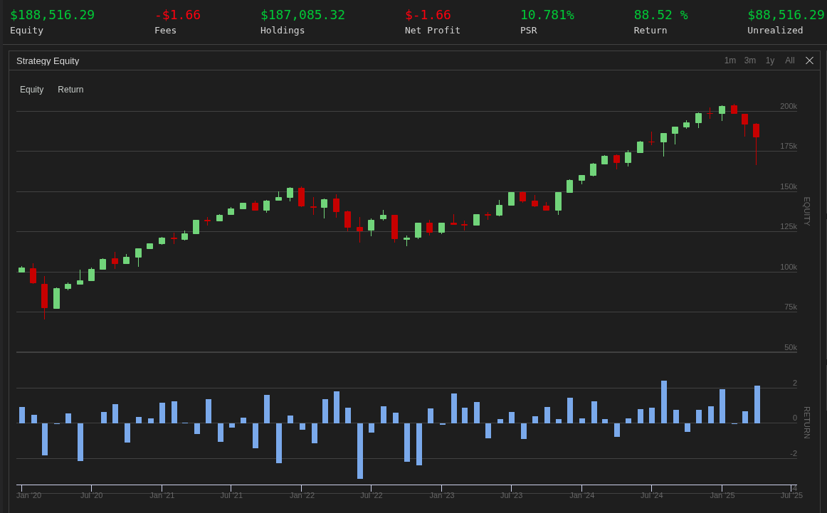
In contrast, the low-volatility strategy not only matched SPY’s total return, but did so with dramatically lower drawdowns (15%) and a Sharpe ratio of 0.73. This confirms that risk-managed equity portfolios can outperform their benchmark with far greater stability.
4. Five Takeaways from the Volatility Strategy
Lower risk can outperform
High-volatility stocks tend to underperform, not just on a risk-adjusted basis, but often in raw returns as well.Simple metrics work
Historical volatility is an intuitive and effective signal. No complex models or machine learning required.Concentration adds value
A portfolio of just 30 names was sufficient to match — and improve upon — the benchmark.Timing matters
Monthly rebalancing reduces turnover and noise compared to daily or weekly approaches.Drawdown control is critical
A trailing stop-loss and portfolio-level cap helped preserve capital during market stress.
5. Strategy Code — Powered by QuantConnect
Below is the simplified monthly selection logic:
    def CoarseSelectionFunction(self, coarse):
        # Limit selection to once per month
        if (self.Time - self.last_selection_time).days < 30:
            return Universe.Unchanged

        self.last_selection_time = self.Time

        # Filter for price > $5 and high volume
        filtered = [x for x in coarse if x.HasFundamentalData and x.Price > 5]
        sorted_by_volume = sorted(filtered, key=lambda x: x.Volume, reverse=True)[:500]
        symbols = [x.Symbol for x in sorted_by_volume]

        # 60-day historical volatility
        history = self.History(symbols, 60, Resolution.Daily)
        if history.empty:
            return []

        vol_dict = {}
        for symbol in symbols:
            if symbol not in history.index.levels[0]:
                continue
            close = history.loc[symbol]['close']
            if len(close) < 60:
                continue
            returns = close.pct_change().dropna()
            vol = returns.std() * np.sqrt(252)
            vol_dict[symbol] = vol

        # Select 30 lowest-volatility stocks
        sorted_vols = sorted(vol_dict.items(), key=lambda x: x[1])[:30]
        self.selected_symbols = [s[0] for s in sorted_vols]

        self.Debug(f"{self.Time.date()} - Selected: {[str(s) for s in self.selected_symbols]}")
        return self.selected_symbols
The initial code was generated by QuantCoderFS (coding flow v1.1) using GPT-4.1, based on the academic literature cited below. It compiled successfully on the first attempt, with a single logic flaw corrected by GPT-4o. Final refinements — including reduced trading frequency and layered risk management — were performed by the author.
Conclusion
This practical test confirms that lower-risk stocks can deliver strong, market-like returns with materially better downside protection. While volatility-based investing may lack the narrative appeal of deep value or high momentum strategies, it offers a disciplined, empirically sound framework for long-term portfolio construction.
References
Blitz, David C. & van Vliet, Pim. (2007). "The Volatility Effect: Lower Risk without Lower Return." ERIM Report Series Research in Management, ERS-2007-044-F&A, Erasmus Research Institute of Management (ERIM), Erasmus University Rotterdam.
Ang, Andrew and Hodrick, Robert J. and Xing, Yuhang and Zhang, Xiaoyan, The Cross-Section of Volatility and Expected Returns. Available at SSRN: https://ssrn.com/abstract=681343
Baker, Nardin L. and Haugen, Robert A., Low Risk Stocks Outperform within All Observable Markets of the World (April 27, 2012). Available at SSRN: https://ssrn.com/abstract=2055431 or http://dx.doi.org/10.2139/ssrn.2055431
Blitz, David and van Vliet, Pim and Baltussen, Guido, The Volatility Effect Revisited (August 26, 2019). The Journal of Portfolio Management, 46(2). , Available at SSRN: https://ssrn.com/abstract=3442749 or http://dx.doi.org/10.2139/ssrn.3442749
S.M.L.